Day 24: Only Circular Shapes

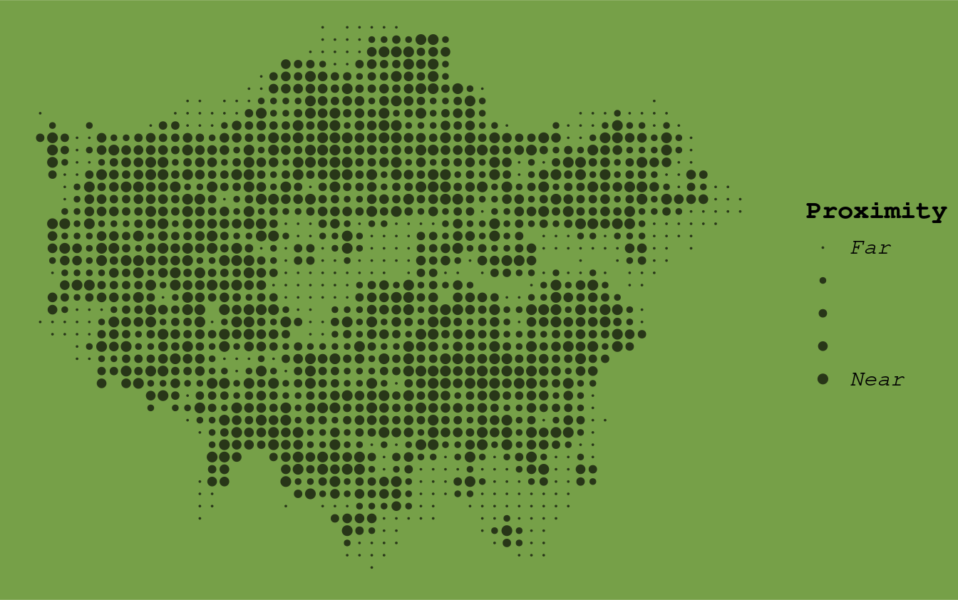
In this map we explore the geography of greenspace in Greater London. Circles are used to visualise change in access. The data used for this map were derived OS Open Greenpace, which were used to generate statistics for a grid of circles spanning Greater London.

First we start by loading the necessary packages:

library(tidyverse) 
library(sf)
library(ggplot2) 
library(magrittr)
library(units) 
library(magick)

Next, we import the greenspace data:

#Load the Greenspace Polygon Data
London_Greenspace <- st_read("London_Greenspace.gpkg",quiet = TRUE)

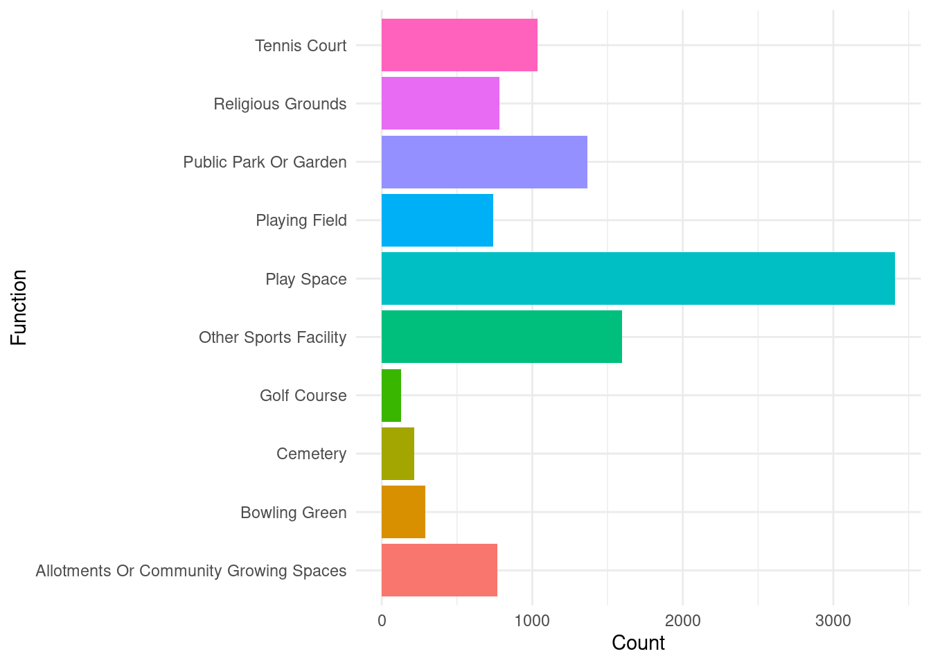
We can have a quick look, both frequency of polygons:

London_Greenspace %>%
 count(function.) %>%
  ggplot(aes(x = function., y = n, fill = function.)) +
   geom_bar(stat = "identity") +
  coord_flip() +
  labs(x = "Function", y = "Count") +
  theme_minimal() +
  theme(legend.position = "none")

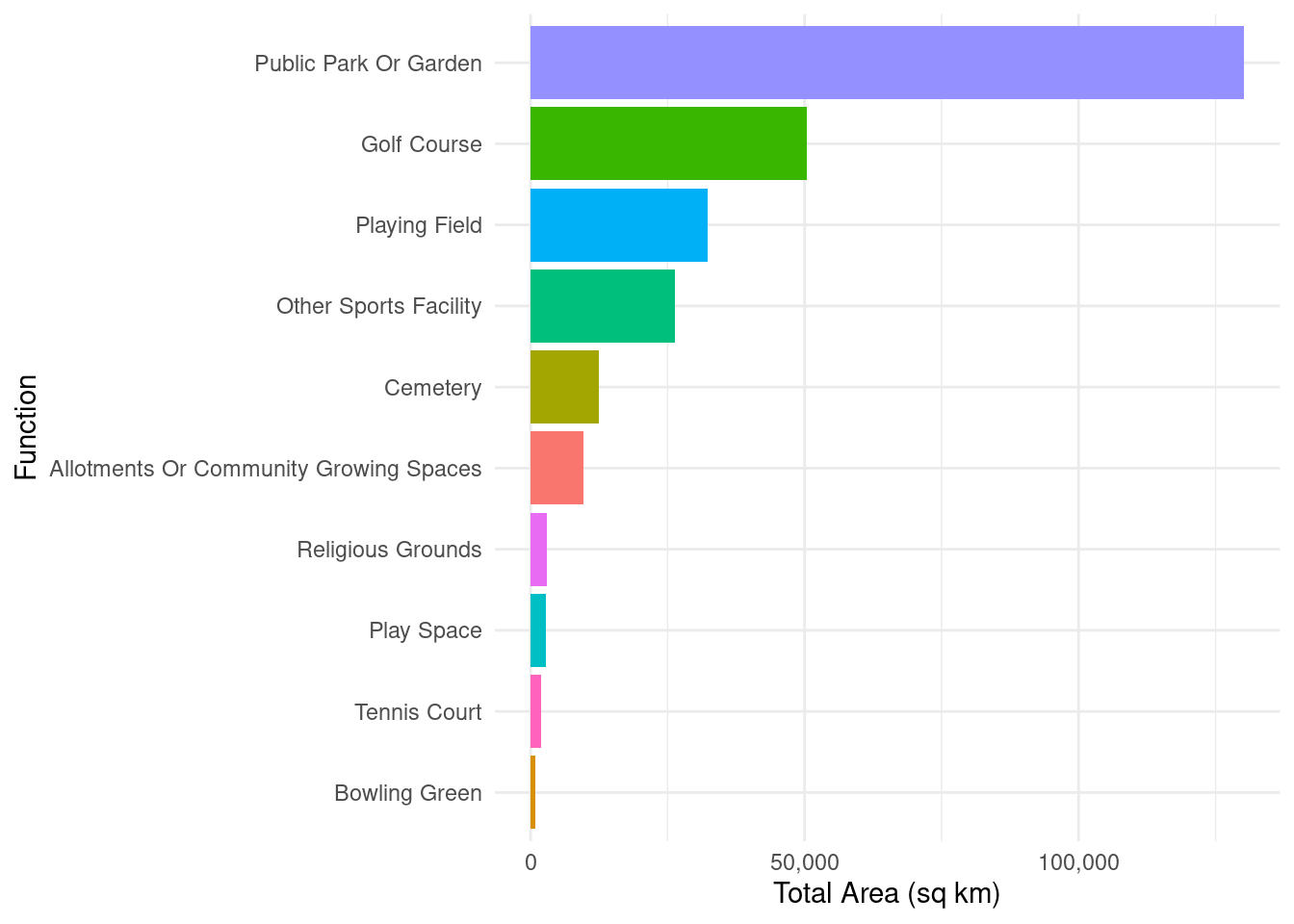
And also the size of the area covered by each category:

# Calculate the area
London_Greenspace <- London_Greenspace %>%
  mutate(area = as.numeric(st_area(geom)))

London_Greenspace %>%
  group_by(function.) %>%    
  summarize(total_area = sum(area, na.rm = TRUE)/1000) %>%
  ggplot(aes(x = reorder(function., total_area), y = total_area, fill = function.)) +
  geom_bar(stat = "identity") +
  coord_flip() +
  labs(x = "Function", y = "Total Area (sq km)") +
  scale_y_continuous(labels = scales::comma) +  
  theme_minimal() +
  theme(legend.position = "none")

Next we will generate a grid of points spanning the extent of London:

# Load the polygon data from the Geopackage
London <- st_read("London.gpkg",quiet = TRUE)

# Create a grid of points within the bounding box of the polygon
grid_points <- st_make_grid(London, cellsize = 1000, what = "centers") %>%
  st_sf()

# Clip the points to only those within Greater London
grid_points <- st_intersection(grid_points, London)

We can then create a subset of the greenspace SF to look specifically at the “Allotments Or Community Growing Spaces” category. Using this, we can then calculate a simple measure of accessibility to these locations from across Greater London.

Allotments <- London_Greenspace %>%
  filter(function. == "Allotments Or Community Growing Spaces")

The following code calculates the distance to the nearest “Allotments Or Community Growing Spaces” polygon for each of the gridded points.

# Calculate the distance from each grid point to the nearest polygon
grid_points <- grid_points %>%
  rowwise() %>%
  mutate(
    distance_to_polygon = min(st_distance(geometry, Allotments))
  ) %>%
  ungroup()

The following code then creates a set of five bins for the distances.

grid_points %<>%
    mutate(distance_category = ntile(-distance_to_polygon, 5))

These are then used to create the map:

ggplot() +
  geom_sf(data = grid_points, color = "#283618", aes(size = distance_category)) +
  scale_size_continuous(
    range = c(0, 2),
    labels = c("Far", "", "", "", "Near")
  ) +
  labs(size = "Proximity") +  # Change "New Legend Title" to your desired title
  coord_sf(crs = st_crs(27700)) +
  theme_minimal() +
  theme(
    axis.text = element_blank(),
    axis.ticks = element_blank(),
    axis.title = element_blank(),
    panel.grid.major = element_blank(),
    panel.grid.minor = element_blank(),
    panel.spacing = unit(0, "mm"),
    plot.margin = unit(rep(0, 4), "mm"),
    #panel.background = element_rect(fill = "#76a048", colour = "#76a048"),
    plot.background = element_rect(fill = '#76a048', colour = '#76a048'),
    legend.text = element_text(size = 12, family = "Mono", face = "italic"),
    legend.title = element_text(size = 14, family = "Mono", face = "bold")
  )