Day 27: Micromapping

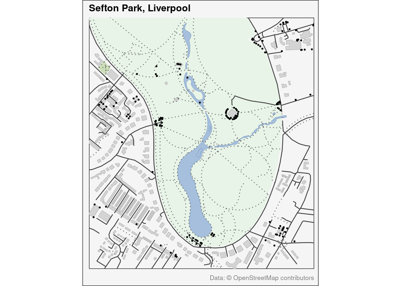
Sefton Park is my nearest large park in Liverpool and very popular. I have not tended to use R to make maps that aren’t data visualisations, so I used todays challenege to create somethign more cartographically orientated.

library(tidyverse)
library(osmdata)
library(sf)
library(ggplot2)

Defining the Area

# Define the bounding box for Sefton Park
bbox <- c(xmin = -2.945, ymin = 53.375, 
          xmax = -2.930, ymax = 53.385)

Downloading OpenStreetMap Data

# Create the query
query <- opq(bbox = bbox)

# Get all relevant features
# Parks and green spaces
parks <- query %>%
  add_osm_feature(key = "leisure", value = "park") %>%
  osmdata_sf()

grass <- query %>%
  add_osm_feature(key = "landuse", value = "grass") %>%
  osmdata_sf()

garden <- query %>%
  add_osm_feature(key = "leisure", value = "garden") %>%
  osmdata_sf()

allotments <- query %>%
  add_osm_feature(key = "landuse", value = "allotments") %>%
  osmdata_sf()

# Water features
water <- query %>%
  add_osm_feature(key = "natural", value = "water") %>%
  osmdata_sf()

# Buildings and infrastructure
buildings <- query %>%
  add_osm_feature(key = "building") %>%
  osmdata_sf()

# Roads - more comprehensive categorization
primary_roads <- query %>%
  add_osm_feature(key = "highway", value = c("primary", "primary_link")) %>%
  osmdata_sf()

secondary_roads <- query %>%
  add_osm_feature(key = "highway", value = c("secondary", "secondary_link")) %>%
  osmdata_sf()

tertiary_roads <- query %>%
  add_osm_feature(key = "highway", value = c("tertiary", "tertiary_link")) %>%
  osmdata_sf()

residential_roads <- query %>%
  add_osm_feature(key = "highway", value = c("residential", "living_street", "unclassified")) %>%
  osmdata_sf()

service_roads <- query %>%
  add_osm_feature(key = "highway", value = "service") %>%
  osmdata_sf()

paths <- query %>%
  add_osm_feature(key = "highway", value = c("footway", "path", "track", "steps", "pedestrian")) %>%
  osmdata_sf()

# Additional features
amenities <- query %>%
  add_osm_feature(key = "amenity") %>%
  osmdata_sf()

leisure <- query %>%
  add_osm_feature(key = "leisure") %>%
  osmdata_sf()

Next we can create the map as a series of layers…

# Create the base map
ggplot() +
  # Base layer - background
  geom_sf(data = parks$osm_polygons,
          fill = "#E8F4E8",  # Light green background
          color = NA) +
  
  # Green spaces
  geom_sf(data = grass$osm_polygons,
          fill = "#CCDEB8",  # Lighter green for grass
          color = NA) +
  
  geom_sf(data = garden$osm_polygons,
          fill = "#C8FACC",  # Slightly different green for gardens
          color = NA) +
  
  geom_sf(data = allotments$osm_polygons,
          fill = "#E4E4E4",  # Grey for allotments
          color = "#C8C8C8") +
  
  # Water features
  geom_sf(data = water$osm_polygons,
          fill = "#A5BFDD",  # Light blue for water
          color = "#819CBD") +
  
  # Buildings
  geom_sf(data = buildings$osm_polygons,
          fill = "#D4D4D4",  # Grey for buildings
          color = "#A9A9A9") +
  
  # Roads - all in dark grey with different widths for hierarchy
  geom_sf(data = primary_roads$osm_lines,
          color = "#424242",  # Dark grey
          size = 1.2) +
  
  geom_sf(data = secondary_roads$osm_lines,
          color = "#424242",
          size = 1.0) +
  
  geom_sf(data = tertiary_roads$osm_lines,
          color = "#424242",
          size = 0.8) +
  
  geom_sf(data = residential_roads$osm_lines,
          color = "#424242",
          size = 0.6) +
  
  geom_sf(data = service_roads$osm_lines,
          color = "#424242",
          size = 0.4) +
  
  # Paths
  geom_sf(data = paths$osm_lines,
          color = "#666666",  # Lighter grey for paths
          size = 0.3,
          linetype = "dotted") +
  
  # Amenities (points)
  geom_sf(data = amenities$osm_points,
          color = "#000000",
          size = 0.5) +
  
  # Coordinate system and bounds
  coord_sf(xlim = c(bbox["xmin"], bbox["xmax"]),
          ylim = c(bbox["ymin"], bbox["ymax"])) +
  
  # Labels and styling
  labs(title = "Sefton Park, Liverpool",
       caption = "Data: © OpenStreetMap contributors") +
  
    theme_minimal() +
  
  # Theme customization
  theme(plot.title = element_text(size = 12, face = "bold"),
        plot.caption = element_text(size = 8, color = "grey50"),
        panel.grid = element_blank(),
        panel.background = element_rect(fill = "#F5F5F5"),
        plot.background = element_rect(fill = "#F5F5F5"),
        # Remove all axis elements
        axis.text = element_blank(),
        axis.ticks = element_blank(),
        axis.title = element_blank())